Identifying and removing or identifying duplicates is one of the essential steps in data cleaning. Duplicates can happen in your data set for many reasons like the nature of the data collection method, data entry errors, etc… This post will show you how to find duplicates in Google Sheets and remove them.
You may also be interested in The Ultimate Guide to Handle Duplicates in Excel.
Table of Contents
Visualizing duplicates in Google Sheets
First of all, you need to visualize the duplicate data in your dataset. This lets you get an idea about the extent of the duplicate data. And also, you can get some idea about the reasons for occurring duplicate data. You may also be able to identify some patterns in the duplicate data. This will help you to decide the techniques for removing duplicate data or separating unique data.
You can easily visualize duplicate data by highlighting them using Google Sheets conditional formatting.
You need to use a custom formula for the format rules in order to highlight duplicates using conditional formatting. These custom formulas are mainly built using the COUNTIF or COUNTIFS functions. I will show you several instances that you may find when working with data.
Highlight duplicates in a single column
Let’s say you have a customer orders list, and some of the order numbers are repeated in the list. You can highlight these repeated order numbers using Google Sheets conditional formatting as explained below.
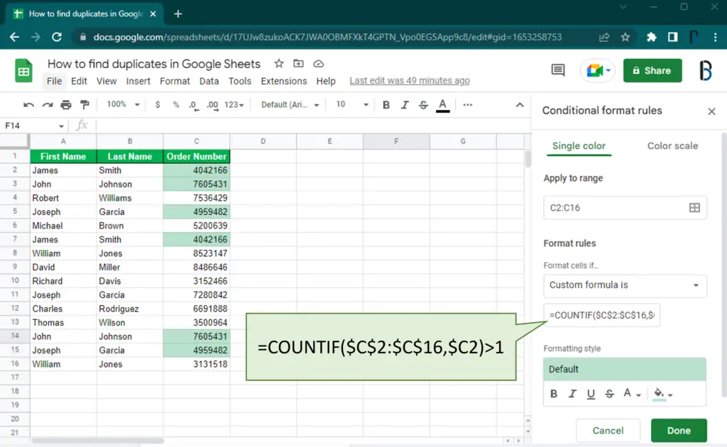
- First, select the column where you need to highlight the duplicates. (i.e. C2:C16)
- Then go to Format > Conditional Formatting.
- You can see that your selected range is included in the “Apply to range” field. You need to enter the correct range otherwise.
- Then under the “Format rules“, for the “Format cells if…” field, select the “Custom formula is” option.
- Then type the following formula in the text box just below the “Format cells if…” field. and click Done.
=COUNTIF($C$2:$C$16,$C2)>1
You need to modify the equation according to your data range. Please ensure that you have put the $ signs as shown in the above example.
The above formula loop through each cell starting from C2 and counts the number of cells that matches the lookup cell. Then if it founds a matching cell or more, it highlights them all.
Highlight duplicate rows in Google Sheets
A complete carbon copy of a record can appears multiple times in the data set. This is the most common type of duplicate issue. You can use the conditional format to highlight these types of duplicates also.
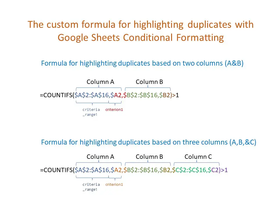
When comparing the entire row, we need to consider all the columns in the data set. So, you need to use the COUNTIFS function instead of the COUNTIF function. The following custom formula matches the entire row (all three columns of the previous example) to find duplicates. You can follow the same steps mentioned above and replace the equation with the following to find duplicates based on the entire row.
=COUNTIFS($A$2:$A$16,$A2,$B$2:$B$16,$B2,$C$2:$C$16,$C2)>1Hint: Build the above COUNTIFS formula inside a cell as you normally write formulas and test it. Then copy and paste the formula for the custom formula textbox.
The following video demonstrates how to highlight duplicate rows in Google Sheets.
Highlight duplicates in Google Sheets multiple columns
You can use the above formula used for highlighting the duplicate rows to highlight duplicates based on multiple columns. When highlighting the duplicate rows, we wrote separate criteria for each column in the dataset. If you write the criteria only for selected columns, it will find and highlight the rows based on those columns only. The following image shows how to use this formula to highlight duplicates in multiple columns.
The following video demonstrates how to highlight duplicates based on multiple columns.
Identify duplicates with Google Sheets Data Cleanup Suggestions
Google is continuously adding smart features to Google Sheets. With Google Sheets Cleanup Suggestions, you can easily identify several issues in your data set before beginning your analysis.
Cleanup Suggestions capable of identifying duplicates in your dataset. To view suggestions,
- Select your data set.
- Go to Data > Data cleanup > Cleanup suggestions. This will open the Cleanup suggestions sidebar and show you the list of duplicates. You can use the same to remove the duplicates.
You can also go to the “Review column stats” link underneath to view more stats column by column.
How to count duplicates in Google Sheets
When dealing with duplicates, you may need to know how many times each data appeared in the list.
Use COUNTIF and COUNTIFS functions to count duplicates
You can use the COUNTIF or COUNTIFS function to count how many times a particular data appears in the range. You can use this for a single column as well as multiple columns.
You can use the following formulas to count duplicates in single columns and multiple columns in Google Sheets. You need to include these function in a new helper column and drag it down until the last row of the data range. It will display the number of occurrences for each row of data.
Ex: Count duplicates in a single column.
=COUNTIF($A$2:$A$16,A2)Ex: Count duplicates based on three columns.
=COUNTIFS($A$2:$A$16,A2,$B$2:$B$16,B2,$C$2:$C$16,C2)Count duplicates using Google Sheets QUERY function
In the previous method, the duplicate count is shown in front of each row. Sometimes it is not easy to find useful information when there is a large number of rows.
With the QUERY function, you can create a summary table with duplicate counts. The “group by” clause can be used to group the identical cells and the “count” aggregate function can be used to count the number of items grouped.
The following formula is group (group duplicates) data based on the A and B columns. And it counts the number of rows grouped and displays them in a new column.
=QUERY(A1:C16,"select A,B,count(B) group by A,B",1)Similarly, the following formula group duplicates considering all A, B, and C columns. Then it displays the number of rows grouped in a new column,
=QUERY(A1:C16,"select A,B,C,count(B) group by A,B,C",1)The following video demonstrates how to count duplicates with the Google Sheets Query function.
How to eliminate duplicates and separate only unique data in Google Sheets
If you disregard the count column in the previous example, other columns represent the list of unique data in your data set.
However, using the UNIQUE function you can get the same result more easily.
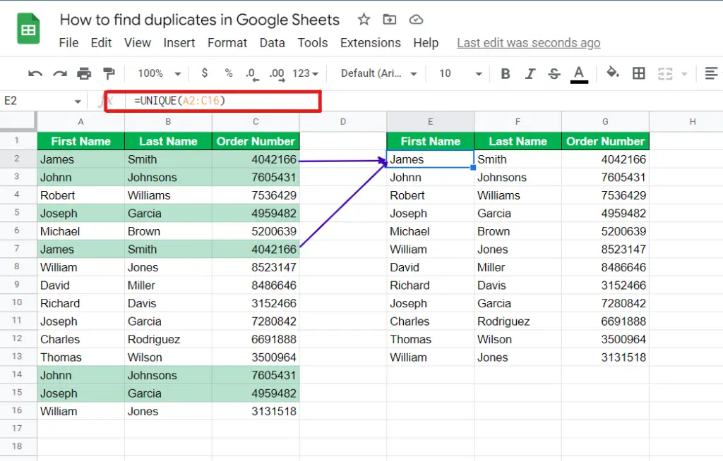
The UNIQUE function has three parameters. By default the second and third parameter is false. To get only UNIQUE records (if there are duplicates, return only one of them) you can forget about the second and third parameters and simply use the function as follows.
=UNIQUE(A2:C16)In the following image, you can see that the unique list includes only one record for duplicate records.
How to extract entries with no duplicates in Google Sheets
In the previous section, we did not consider the second and third parameters of the UNIQUE function.
The function looks for duplicate columns if you put “TRUE” as the second parameter and, it eliminates duplicate columns if available.
By default, the third parameter is also “FALSE”. If you put “TRUE” for the third parameter, it returns only the record with no duplicates. You can use the equation shown below to return records with no duplicates.
=UNIQUE(A2:C16,,TRUE)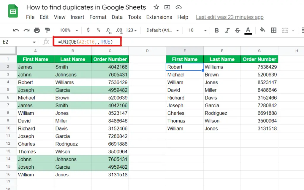
How to remove duplicates in Google Sheets
Previously, we generated a separate unique list while keeping the original data untouched. That is more safe method since you are not losing any rows in the original data set.
If you want to completely remove the duplicates from your data set,
- Select your data set.
- Go to Data > Data cleanup > Remove duplicates.
- If you have selected header rows, check the “Data has header row” checkbox.
- Then you can select based on which column you need to find duplicates. Select all columns if you want to remove duplicate rows considering all columns.
Wrapping Up
Identifying and removing duplicates is an essential step in preparing your dataset for analysis. Interestingly there are several methods to handle duplicates in Google Sheets.
In this post, we discussed how to highlight duplicates using conditional formatting. You can highlight duplicates on a single column as well as on multiple columns or duplicate rows. Then we discussed how to count duplicates and create a summary table with duplicate counts.
We also discussed how to extract unique data and entries with no duplicates from your data set. And finally, we discussed how to remove duplicates in Google Sheets.
