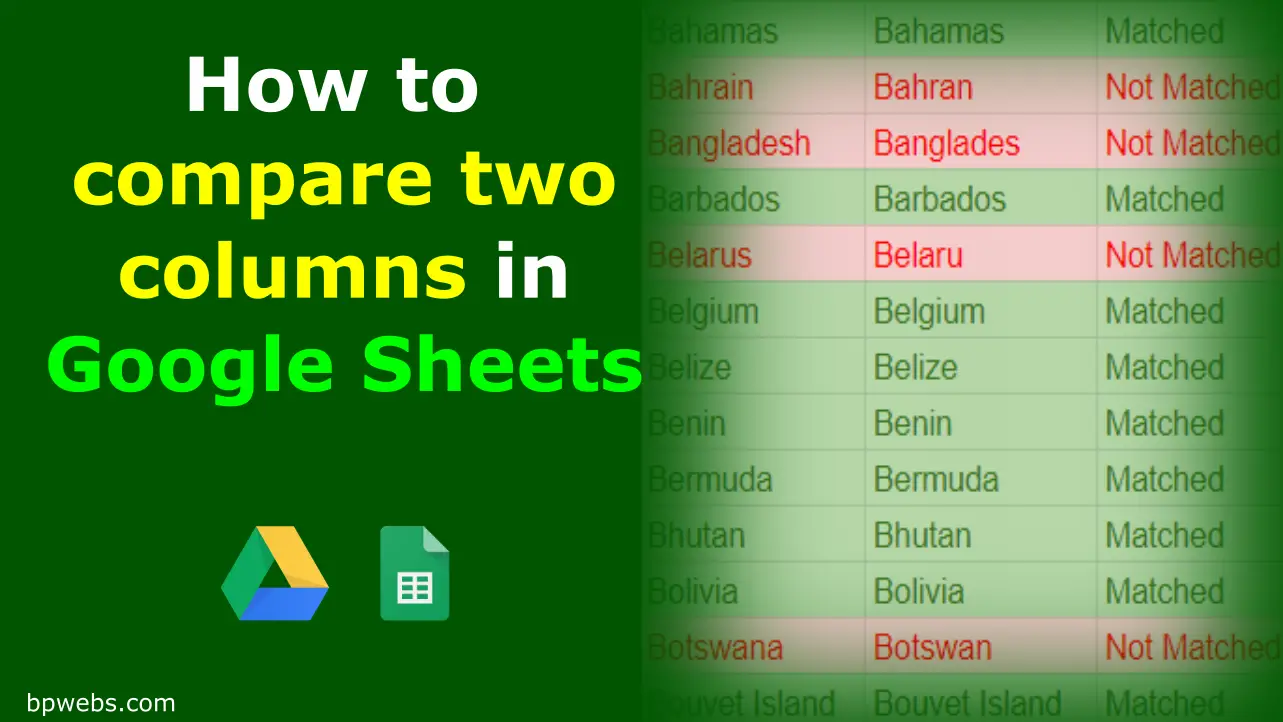
When working with data, you may come across situations where you need to compare two or more datasets. For example, you may need to compare two different versions of the same data set. In such situations, we can compare the data sets using individual columns or column combinations. This post will show you how to compare two columns in Google Sheets. And, you will learn how you can compare two datasets using these techniques.
You may need to run the comparison process multiple times. You can simply start comparing the datasets with basic formulas. If you found only a few non-matching data, you can look at them manually. If not, you need to perform some other techniques such as removing extra spaces, cleaning, splitting into columns, etc…
In this post, we will discuss a set of useful techniques that you can use to compare two columns in your Google Sheets. The steps are not in order, so you can use them interchangeably.
Table of Contents
Clean up the data
Using data entry forms for collecting data can reduce human errors.
Your data may not match due to small differences, such as multiple spaces, changes of letters or non-printable characters, etc…
If you have non-matching data in the two columns you are comparing, you can apply the following data cleaning techniques to both data sets separately. Then again you can compare the two columns.
Remove multiple spaces
If one of your records has multiple spaces at the beginning, middle or end, the spreadsheet recognizes them as two different records. As such, you should trim those unnecessary multiple spaces before comparing such data.
You can use the TRIM function in Google Sheets to remove multiple spaces in your records. Both of your columns may contain such records with multiple spaces. So, you should trim both columns.
Syntax: TRIM(Text)
Example: TRIM (” lorem ipsum “) returns “lorem ipsum”
Remove non-printable characters
Your data may contain nonprintable characters such as tabs, line breaks, etc… If one of your data has such characters, it does not match with the other.
You can remove nonprintable characters using the Google Sheets CLEAN function.
Syntax: CLEAN(text)
By using this function, you will not see any visible changes in your text as the Google Sheet does not show nonprintable characters.
Replace part of the text
Sometimes, your data may be mismatched due to small changes in a sentence or word.
For example, in some countries, people’s names end with the letter “a” or “e”. In one column you may have the name ends with the letter “a” and the other has the letter “e”.
In such a situation, you can replace the last letter with one of those before comparing the two columns.
For this, you can use the REPLACE function in Google Sheets.
Syntax: REPLACE(text, position, length, new_text)
Compare two columns in Google Sheets by comparing cells in the same row
Let’s say you have the same number of records in both columns. In such cases, you can use the method described below to compare two columns by comparing the cells in the same row.
Compare data using the equal (“=”) operator
You can compare two records for equality using the equal (“=”) operator.
For example, if you want to compare cells A2 and B2 you can use the following equation on another cell (i.e. C2)
=A2=B2
If the two records are matched it returns TRUE, and FALSE otherwise.
This equation is useful when you have the same number of rows in both columns and you only need to compare the records in the same row. You cannot use this to compare cross rows.
Modify the equation to return a pre-defined term
The above equation returns TRUE or FALSE depending on the situation. However, TRUE/FALSE are not familiar terms for some people. Therefore, you can modify the equation as below to return meaningful terms instead of TRUE/FALSE.
=IF(A2=B2,"Matched","Not Matched")
Highlight matching data in two columns
Sometimes we need to visually see the differences in the two columns. This helps you to make quick decisions regarding the two data sets.
You can compare and highlight matching records in two columns using Google Sheets conditional formatting.
To highlight matching records with Conditional formatting,
- First, select the data range (the two columns, i.e. A2:B10) then go to Format > Conditional formatting. In the “Single color” tab, make sure the “Apply to range” is correct.
- Under the “Format rules” for the “Format cells if…” select the “Custom formula is“
- If you are to compare columns A and B, enter the formula
=$A2=$B2in the “Value or formula” text box. - Then select the formatting styles and click Done.
If you want to highlight the data that does not match, you can use the following formula,
=$A2<>$B2
Compare two columns of different sizes
The previous method is suitable to compare columns of the same size. When you have unordered two lists of different sizes that method cannot be used.
Compare columns with the VLOOKUP function
For this, you can use the VLOOKUP function to compare the two columns.
If you want to check what records of one column appeared in the other column, you can use a formula similar to the one below.

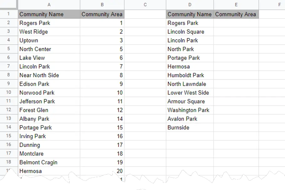
In the above image, let’s say you want to check whether all the Community Names in the table on the right side are included in the left side table. You can place the following formula in cell E2 and drag it down.
=iferror(VLOOKUP(D2,$A$2:$B$75,2,false),"Not Found")
Then it will show the community area number in front of the name and shows the text “Not Found” otherwise (See the short video below).
Compare columns using the COUNTIF function
When comparing two columns you can use the COUNTIF function to count how many times a record in one column appeared in another column.
Let’s say you need to compare columns A and B. And, you want to check which records in column B appeared in column A and how many times. In this case, you can use the COUNTIF function.
For example, the following equation compares the record in cell B2 with records in range A2:A21. It returns the number of times that record in cell B2 appeared in the range A2:A21.
=COUNTIF($A$2:$A$21,B2)
Compare column combinations or complete rows
In some cases, we cannot be satisfied by comparing one column. In such cases, we can create a single column by combining the required or all columns in both data sets separately. Then we can perform the comparison methods described above on combined columns.
You can use the CONCATENATE function to combine multiple columns into one.
The following formula combines the content in A2, B2, and C2 cells into one string.
=CONCATENATE(A2,B2,C3)
Wrapping Up
In this post, we discussed several methods that you can use to compare two columns in Google Sheets. It also discussed several methods to prepare and clean the data sets before the comparison. You can use these methods to compare two different data sets or two versions of the same data set to make some decisions.
