How to create dropdown lists in Excel (Dependent & Multirow)

In this article, I will show you how to create dropdown lists and dependent dropdown lists in Excel and apply them to multiple rows. Dropdown lists allow users to select from a list of options when entering data into a cell. This can help to ensure that data is entered correctly and consistently. Dependent dropdown lists are a type of dropdown list that changes the available options based on the selection made in another dropdown list. This can be useful for creating forms or tables where the options in one field depend on the selection made in another field. By following the steps in this article, you will be able to create dropdown lists and dependent dropdown lists in Excel that can help you improve the accuracy and consistency of your data entry.

Video Tutorial

If you’d prefer written instructions, just keep reading.

When do you need dropdown lists in Excel?

Basically, in Excel, a dropdown list is a part of data validation and is useful in many ways. Here are a few of the most common uses,

• To limit the number of choices available to the user. This can help to ensure that data is entered consistently and accurately. For example, you could use a dropdown list to restrict the values that can be entered into a cell to a list of valid product codes.
• To prevent spelling mistakes. When users select a value from a dropdown list, they are less likely to make a spelling mistake than if they had to type the value in manually. This can help to improve the accuracy of your data.
• To make data entry faster. Instead of having to type in a value, users can simply select it from a dropdown list. This can save time and make data entry more efficient.
• To add a level of interactivity to your spreadsheet. Drop-down lists can be used to create interactive forms, menus, and dashboards. This can make your spreadsheet more user-friendly and engaging.

How to create dropdown lists in Excel

Creating a single dropdown list in Excel is straightforward. To do that, follow these steps:

1. Select the cell where you want the dropdown list to appear.
2. Go to the Data tab on the ribbon.
3. In the Data Tools group, click Data Validation.
4. In the Data Validation dialog box, select List from the Allow dropdown list.
5. In the Source box, type or select the data range you want to appear in the dropdown list.
6. Click Ok.

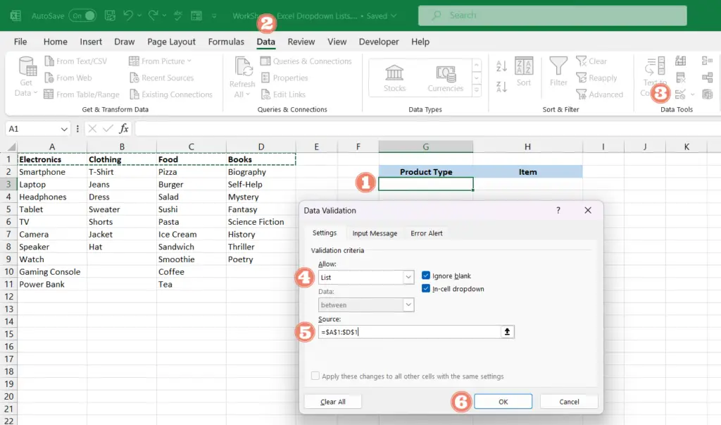
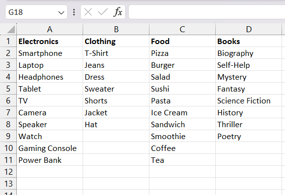
In Figure 1 above, you can see that we have a list of data in the A, B, C, and D columns. The first row contains the product types and right below there are list of items under each product type. In the above steps, we created a product dropdown list from this dataset by selecting the range A1:D1 for the Source box of the Data Validation dialog box.

How to create dependent dropdown lists in Excel

Dependent dropdown lists are a type of dynamic dropdown list that changes the available options based on the selection made in another dropdown list.

Let’s say, for example, that you have created an item dropdown from the list of items in all A, B, C, and D columns shown in Figure 1 above. This approach makes the list unnecessarily lengthy, and users will find it difficult to select the correct item.

Instead of creating a list dropdown using all the list items, you can create a primary dropdown list for “product types” and a dependent dropdown list for ‘items“. With this, you can populate the items dropdown list only with items belonging to the selected Product item.

For this setup, you can use the dropdown list created above as the Primary Dropdown list.

Before creating the dependent dropdown list, we need to name the ranges of four item lists in the A, B, C, and D columns from their product names using Excel’s Named Range feature.

Name the ranges used for the dependent dropdown list

We need to name each range by their product type. For example, use the name “Electronics” to name the list of items under the Electronic product type.

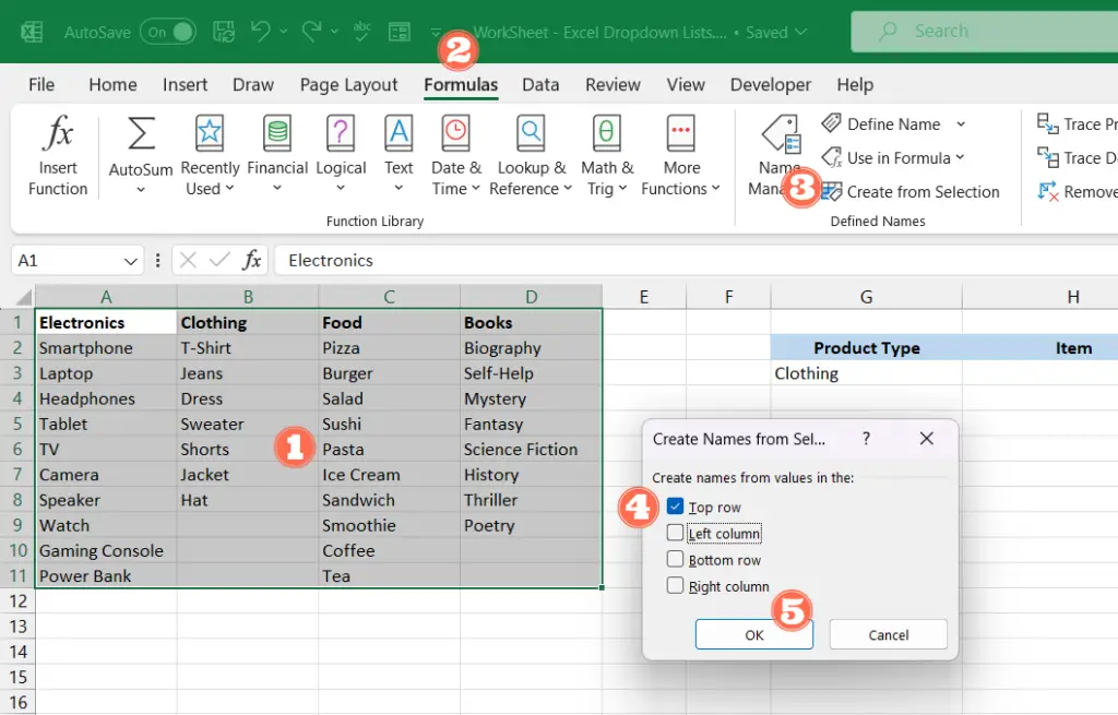
You can easily do this with the “Create from selection” option of the Defined name group in the Formulas tab. Here is how;

1. Select the entire data range (i.e. A1:D11)
2. Go to the Formulas tab
3. Click the “Create from Selection” button in the Defined Names group
4. Leave only the “Top row” check box checked.
5. Click Ok.

Now you can check the named ranges by going to the named box on the left side of the formula bar. Once you click the down arrow, you will see a list of names such as, “Electronics”, “Clothing”, “Food”, and “Books”. You can select the name and see the range that it applies to.

Create the dependent dropdown List

Now everything is ready to create the dependent dropdown list. To create it;

1. Select the cell where you want the dependent dropdown list to appear.
2. Go to the Data tab on the ribbon.
3. In the Data Tools group, click Data Validation.
4. In the Data Validation dialog box, select List from the Allow dropdown list.
5. In the Source box, type the formula =INDIRECT(G3), where cell G3 contains the primary dropdown list.
6. Click Ok.

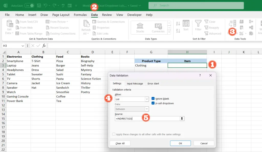
Now your dependent dropdown is ready. You can test it by changing the value in the primary dropdown list.

How to remove blank options in the dependent dropdown list

When creating named ranges, we selected all lists together. However, if certain ranges have fewer items, your dependent dropdown for that category may contain empty items. To eliminate these blank items, you should edit the named range to exclude the empty cells using the Name Manager. Alternatively, you can select the columns one by one when defining named ranges. This way, you can ensure that empty cells are excluded from the range right from the beginning.

How to apply this dropdown and dependent dropdown to multiple rows

You can easily copy these dropdowns to any location on the sheets. Since we’ve utilized absolute references and named ranges, they function as intended across the entire sheet. Just drag down or copy-paste the dropdowns to other rows, much like you would with other formulas, to apply them to multiple rows. If you have copied the dropdowns with already selected data, simply select and delete the content, and your dropdown lists (data validation) will be preserved.

How to highlight invalid data

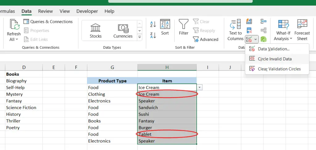
One issue with this type of dependent dropdown list is that if you change the selected item in the primary dropdown later, the selected item in the dependent dropdown list will not be updated. You can identify cells with invalid data of this type by using the “Circle Invalid Data” option. To do this;

1. Select the range of cells for which you suspect invalid data.
2. Go to the Data tab.
3. Click the small down arrow in the Data Validation button.
4. Then select the “Circle Invalid Data” option.

Wrapping Up

In this guide, we explore the creation of dropdown lists and dependent dropdown lists in Excel, extending the functionality to multiple rows. Dropdown lists enhance data entry precision by offering selectable options. Dependent dropdowns, adjusting options based on prior selections, are particularly useful for dynamic forms or tables. By adhering to our step-by-step instructions, you can establish dropdowns and dependent dropdowns that streamline data entry accuracy and consistency. This article elucidates both procedures and imparts valuable insights for managing data in a more organized, accessible, and interactive manner.