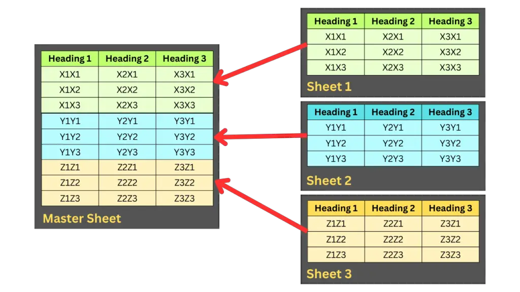
In today’s data-driven world, efficient data management is crucial for individuals and organizations. Google Sheets, a powerful cloud-based spreadsheet tool, offers many features to help users organize, analyze, and visualize data. One valuable technique for managing data across multiple sheets is to create a “Master Sheet.” A Master Sheet consolidates information from different sheets into a single, comprehensive view, making it easier to access and analyze data. In this article, we will guide you through the process of creating a Master Sheet in Google Sheets and explore its benefits.
If you are looking for a quick answer, use the following formula to import data from the source Sheets to the master sheet. You can also continue reading for more detailed information on creating a Master Sheet in Google Sheets.
=QUERY({Sheet1!A2:E;Sheet3!A2:E;Sheet2!A2:E},"select * where Col1 is not null")Table of Contents
Understanding the Concept of a Master Sheet
A Master Sheet is a centralized location where data from various sheets is gathered, eliminating the need to switch between multiple sheets for data analysis. By combining related information into one sheet, you can simplify data management and draw insights more effectively. This approach is particularly useful when working with large datasets, complex projects, or collaborative efforts involving multiple team members.

Benefits of a Master Sheet in Google Sheets
Creating a Master Sheet offers several advantages:
- Streamlined Data Analysis: With all relevant data in one place, analyzing trends, performing calculations, and generating reports become more efficient and accurate.
- Centralized Data Management: Instead of handling data across multiple sheets, you can focus on managing a single Master Sheet, simplifying version control and collaboration.
- Easy Data Updates: Google Sheets’ automatic update feature ensures that your Master Sheet reflects the latest changes from the source sheets without manual intervention. In other words, the master sheet is dynamic.
- Data Integrity: By referencing the original data in the source sheets, you maintain data integrity and minimize the risk of accidental data loss.
- Enhanced Collaboration: A Master Sheet allows multiple team members to access and work with consolidated data simultaneously, fostering collaboration and productivity.
Especially, the dynamic nature of the Master Sheet saves you tons of time by automatically updating the data whenever changes are made in the linked sheets. You won’t have to manually update the formulas each time the source sheets are modified, making data consolidation and analysis much more efficient. Furthermore, rest assured that your original data remains untouched in the source sheets.
How to import data to Master Sheet
Within this post, we have primarily focused on importing data using the built-in Google Sheets functions. You can also use Google Apps Scripts and Triggers to perform more complex tasks.
Using the QUERY function
To perform this task, I am going to use the Google Sheets QUERY() function. The QUERY function in Google Sheets is a powerful tool that can be used to consolidate data from multiple sheets into a Master Sheet. It offers a more flexible and dynamic way to extract and organize data based on specific criteria.
If you haven’t used the QUERY function before, it is highly recommended that you learn how to use it. Mastering this function can significantly enhance your ability to manage and analyze data in Google Sheets efficiently.
The QUERY function can perform several actions that would otherwise require multiple functions. For example, you can use the QUERY function to:
- Select specific columns or rows from a dataset.
- Filter data based on specific criteria.
- Calculate summary statistics.
- Join data from multiple tables.
- Create pivot tables.
The basic syntax of the QUERY function is QUERY(data, query, [headers])
- data refers to the range of cells containing your dataset.
- query represents the conditions or instructions for filtering and sorting your data.
- headers [optional] indicates whether your data has headers or not
The QUERY formula to combine data from multiple ranges to the Master Sheet
To better understand, let’s start with an example. You can make a copy of the Google Sheets with sample data from the following link, or you can use your own.
Copy this Google Sheets Workbook to your drive from this link.

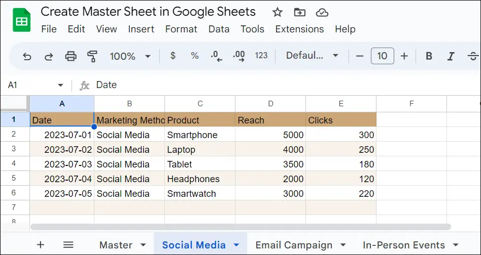
In the above workbook, we have 4 tabs (sheets) namely
- Master (This is the master tab we discuss in this post)
- Social Media (a source tab)
- Email Campaign (a source tab)
- In-Person Events (a source tab)
So, you can use the following formula in the Master tab to import and consolidate all the data from the source sheets into one range.
=QUERY({'Social Media'!A2:E;'In-Person Events'!A2:E;'Email Campaign'!A2:E},"select * where Col1 is not null")
In the above formula, the first part which is inside the curly brackets is used to create a list of ranges in other words an array of data. The list of ranges is then passed to the QUERY function as the data argument.
data = {'Social Media'!A2:E;'In-Person Events'!A2:E;'Email Campaign'!A2:E}
The data received from the source sheets are stacked in the same order you provided the ranges to the above array.
The second part of the formula is the query argument.
query = "select * where Col1 is not null"
In the above query, we instruct the QUERY formula to return all (*) the rows that meet our specified criteria. The criteria we set is represented by the “Col1 is not null” part of the query.
In some cases, you might have encountered column references using column headers such as A, B, etc. However, when combining multiple ranges using curly braces {}, it is necessary to use the Col1, Col2, etc. notation to refer to columns. The Col1, Col2, etc. notation represents the columns of the entire combined range,
We use the “Col1 is not null” condition in the QUERY function to exclude importing empty rows. However, this condition specifically checks only the first column to identify empty rows, assuming that the entire row is empty if the data in the first column is empty. If you want to check for emptiness in other columns, you can modify the condition accordingly. For example, to include rows that have data in either the first, second, or third column, you can use the condition “Col1 is not null or Col2 is not null or Col3 is not null” within the QUERY function. This way, you can tailor the condition to suit your specific data and filter out unwanted empty rows during the import process.
How to create a master sheet for data in different Google Sheets Workbooks
In the previous section, we discussed importing data from different tabs within the same Google Sheets Workbook where the Master Sheet exists. However, you can take data consolidation a step further by importing data from various Google Sheets Workbooks and creating a comprehensive Master Sheet.
To achieve this, you’ll need to use an additional formula called IMPORTRANGE(). The IMPORTRANGE function is a powerful tool in Google Sheets that allows you to import data from one workbook to another. It plays a key role in creating a dynamic Master Sheet that fetches data from multiple sources, keeping your analysis up-to-date and well-organized.
The IMPORTRANGE function facilitates data synchronization between different Sheets, making it incredibly useful when you want to consolidate data from various departments, regions, or projects into a central location for analysis.
Let’s delve deeper into the process of using the IMPORTRANGE function in combination with the QUERY function to create an efficient and dynamic Master Sheet.
The basic syntax of the IMPORTRANGE function is IMPORTRANGE(spreadsheet_url, range_string).
- spreadsheet_url – The URL of the spreadsheet (Workbook) from where data will be imported.
- range_string – A string, of the format “[sheet_name!]range” (e.g. “Sheet1!A2:B6” or “A2:B6”) specifying the range to import.
So, we can write the formula as below.
=IMPORTRANGE("https://docs.google.com/spreadsheets/d/1qgSvyRC6zEQI_aV6xVwe6Xep6vGBfQp-tISdxo7e2-k/edit#gid=1736580271","'Social Media'!A2:E")The output of this formula is a range, so you can use it as the input to another function, including the QUERY function. Let’s consider a scenario where our previous tabs are now in separate Google Sheets workbooks. You can still consolidate data from these different workbooks by leveraging the IMPORTRANGE function and then rewrite the QUERY formula accordingly.
=QUERY({IMPORTRANGE("https://docs.google.com/spreadsheets/d/1HEEovzGWxQKLbHJQcDb0zEMxZOC10XzJvprjdkmQD6k/edit#gid=0","'Social Media'!A2:E");
IMPORTRANGE("https://docs.google.com/spreadsheets/d/1bJooGBHuih8dmaw9R_aQ7JWqGDYKEWVAE6UgsedFPDk/edit#gid=482828263","'In-Person Events'!A2:E");
IMPORTRANGE("https://docs.google.com/spreadsheets/d/1J7EYZKFlrmplDKT4Fj4MaVxZ1jLHxHU6cFlIQkRe9yU/edit#gid=1482938456","'Email Campaign'!A2:E")},
"select * where Col1 is not null")
You can copy and paste the above formula to your Google Sheets to see how it works, or make a copy of the sample Google Sheets workbook from this link.
You may also read: How to import data from one Google Sheet to another
Improve the readability of the formula
The previous query formula can become hard to read, especially since the Google Sheets URL is long. To enhance readability, consider creating a table in the workbook which Master Sheet exist where you can store the URLs of the source sheets. Then, you can reference the cell addresses containing these URLs as arguments for the formula. By doing so, you can significantly improve the formula’s readability and maintainability.
Wrapping Up
Creating a Master Sheet in Google Sheets is an effective way to streamline data management and analysis. By consolidating data from multiple sheets into one centralized location, you can simplify the process of drawing insights, generating reports, and collaborating with others. Whether you’re managing personal projects or working on collaborative team efforts, mastering this technique will undoubtedly enhance your productivity and data handling capabilities in Google Sheets.
To import data from source tabs within the same Google Sheets Workbook to the Master Sheet, you can use the Google Sheets QUERY function. Additionally, by combining the IMPORTRANGE function with QUERY, you can import data from other Google Sheets Workbooks, allowing you to consolidate information from multiple sources effortlessly. This dynamic approach ensures your Master Sheet remains up-to-date, reflecting any changes made in the source sheets in real-time.
In conclusion, the ability to create a Master Sheet in Google Sheets is a valuable skill for anyone dealing with data-intensive tasks. Embrace this powerful technique to efficiently manage and analyze data, bringing convenience and efficiency to your data-driven endeavors.
